It is easy to find simple numerical information on hockey players to use in your Word table and your Excel spreadsheet.
You can go to either
Wikipedia at http://wikipedia.org/
or
The Internet Hockey Database at
http://www.hockeydb.com/
Search for the name of any hockey player, such as
Mats Sundin
Wayne Gretzkly
Boom-Boom Geoffrion
Rocket Richard
Thursday, January 17, 2008
Wednesday, December 19, 2007
Excel - ex. 9
EXERCISE 9 - Inserting Columns & Rows
Your teacher would like you to update the Record of Marks spreadsheet created in exercise 8.
1. Recall the exercise named Excel ex8 to your screen
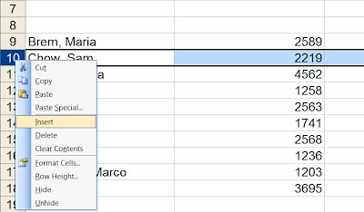
2. Select row 10 and insert a new row using the right mouse.
RIGHT-click on the row header for Row 10, then select Insert.
Enter the data for the first student:
Brown, Jamie 3002; 21; 25; 20

Determine where Johanna should be added alphabetically and insert a new row and enter the data.
Desousa, Johanna 1435; 28; 32; 20
Format and add calculations to the new rows to match the existing rows.

3. Select column E and insert a new column.
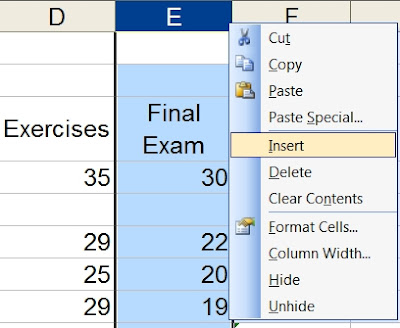
Enter the column heading Assignments. Change the new column width if necessary. Enter the new column values of 40; 32, 30, 35, 28, 22,17, 25, 22, 29, 31, 33,16. Update the cell formats to match the current formats.
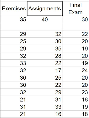
4. Add a new column heading in cell H6 called Student %.
5. In cell H9, calculate the Student % for his/her total mark. The formula to calculate the percent is the Student Total Mark divided by the Total. Set the Total cell as an absolute cell in the formula.
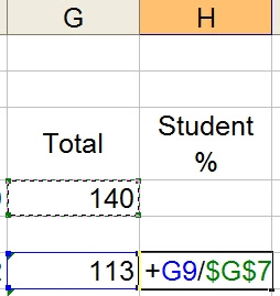
Format the result to % with 0 decimal places. Copy the formula down.
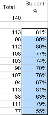
6. At the bottom of the spreadsheet in column A, add 4 new row labels Average Course Mark, Top Course Mark, Low Course Mark and Number of Students.
Use functions that will calculate the above figures for column H only. Format the answers to match the rest of the columns.
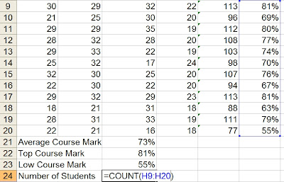
7. Change the page orientation to landscape. Center the spreadsheet horizontally and vertically on the page.
8. IMPORTANT - Use the SAVE AS command to save the spreadsheet file as Excel ex9.
Your teacher would like you to update the Record of Marks spreadsheet created in exercise 8.
1. Recall the exercise named Excel ex8 to your screen
2. Select row 10 and insert a new row using the right mouse.
RIGHT-click on the row header for Row 10, then select Insert.

Enter the data for the first student:
Brown, Jamie 3002; 21; 25; 20

Determine where Johanna should be added alphabetically and insert a new row and enter the data.
Desousa, Johanna 1435; 28; 32; 20
Format and add calculations to the new rows to match the existing rows.

3. Select column E and insert a new column.

Enter the column heading Assignments. Change the new column width if necessary. Enter the new column values of 40; 32, 30, 35, 28, 22,17, 25, 22, 29, 31, 33,16. Update the cell formats to match the current formats.

4. Add a new column heading in cell H6 called Student %.
5. In cell H9, calculate the Student % for his/her total mark. The formula to calculate the percent is the Student Total Mark divided by the Total. Set the Total cell as an absolute cell in the formula.

Format the result to % with 0 decimal places. Copy the formula down.

6. At the bottom of the spreadsheet in column A, add 4 new row labels Average Course Mark, Top Course Mark, Low Course Mark and Number of Students.
Use functions that will calculate the above figures for column H only. Format the answers to match the rest of the columns.

7. Change the page orientation to landscape. Center the spreadsheet horizontally and vertically on the page.
8. IMPORTANT - Use the SAVE AS command to save the spreadsheet file as Excel ex9.
Excel - ex. 8
Exercise 8
Your teacher has asked you to create a spreadsheet that will calculate student marks based upon tests, exercises, and final exams.
1. Enter the spreadsheet values and labels using cells A1 through F18. Format the values and labels as shown. Enter your teacher's name in cell B4.
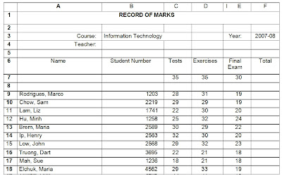
2. Use the AutoSum function to:
• in cell F7 add C7 through E7
• in cell F9 add C9 through E9 and copy the function down to cell F18
3. Highlight range of cells A9 through F18. Sort the list of students alphabetically using the A-Z sort ascending button on the standard toolbar.
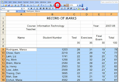
4. Save the spreadsheet as Excel ex8.
5. Add a footer
Your teacher has asked you to create a spreadsheet that will calculate student marks based upon tests, exercises, and final exams.
1. Enter the spreadsheet values and labels using cells A1 through F18. Format the values and labels as shown. Enter your teacher's name in cell B4.

2. Use the AutoSum function to:
• in cell F7 add C7 through E7
• in cell F9 add C9 through E9 and copy the function down to cell F18
3. Highlight range of cells A9 through F18. Sort the list of students alphabetically using the A-Z sort ascending button on the standard toolbar.

4. Save the spreadsheet as Excel ex8.
5. Add a footer
Excel - ex. 7
EXERCISE 7
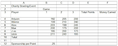
The Jarvis Business Department held a Charity Bowling Event last weekend. They have approached the Introduction to Information Technology students to create a spreadsheet to calculate Total Money Raised. Six students participated in the event and obtained sponsorship from the friends at a rate of 25 cents per bowling point.
Instructions
1. Enter the spreadsheet values and labels using cells A1 :F12.
2. Cell formatting instructions:
o Merge and center the spreadsheet heading using any font size 14
o Merge and center cells B2:D2 for the spreadsheet sub-heading using any font size 8
o Horizontally & vertically center and wrap text the labels in cells A3:F3
o Right align the label in cell A10
o Format cell B12 to currency with 2 decimal places
Calculating instructions:
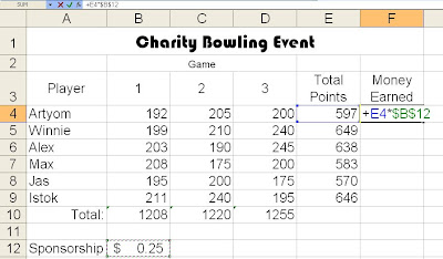
o In cell B10, use the AutoSum button to add the total points per game. Fill the function right to F10
o In cell E4, use the AutoSum button to add total points per player. Fill the function down to E9
o In cell F4, enter a formula to calculate money earned per player. Multiply the total points by the sponsorship rate per point. Use an absolute cell in the formula.
Additional Formatting instructions:
o Add appropriate borders
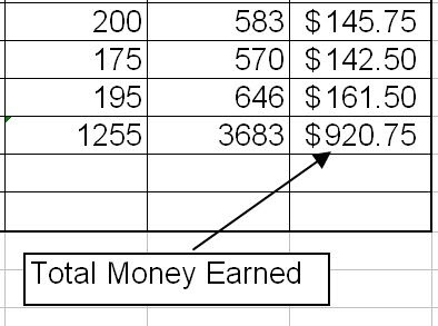
o Add a textbox with the text Total Money Earned and draw an arrow from the textbox to the total figure
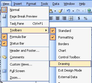
Use VIEW / TOOLBARS / DRAWING to see your Drawing Toolbar.
o Change the page orientation to landscape & center the spreadsheet on the page
o Add a footer & save as Excel ex7
The Jarvis Business Department held a Charity Bowling Event last weekend. They have approached the Introduction to Information Technology students to create a spreadsheet to calculate Total Money Raised. Six students participated in the event and obtained sponsorship from the friends at a rate of 25 cents per bowling point.
Instructions
1. Enter the spreadsheet values and labels using cells A1 :F12.
2. Cell formatting instructions:
o Merge and center the spreadsheet heading using any font size 14
o Merge and center cells B2:D2 for the spreadsheet sub-heading using any font size 8
o Horizontally & vertically center and wrap text the labels in cells A3:F3
o Right align the label in cell A10
o Format cell B12 to currency with 2 decimal places

Calculating instructions:
o In cell B10, use the AutoSum button to add the total points per game. Fill the function right to F10
o In cell E4, use the AutoSum button to add total points per player. Fill the function down to E9
o In cell F4, enter a formula to calculate money earned per player. Multiply the total points by the sponsorship rate per point. Use an absolute cell in the formula.

Additional Formatting instructions:
o Add appropriate borders
o Add a textbox with the text Total Money Earned and draw an arrow from the textbox to the total figure
Use VIEW / TOOLBARS / DRAWING to see your Drawing Toolbar.


o Change the page orientation to landscape & center the spreadsheet on the page
o Add a footer & save as Excel ex7
Subscribe to:
Comments (Atom)