Your teacher would like you to update the Record of Marks spreadsheet created in exercise 8.
1. Recall the exercise named Excel ex8 to your screen
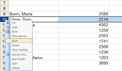
2. Select row 10 and insert a new row using the right mouse.
RIGHT-click on the row header for Row 10, then select Insert.
Enter the data for the first student:
Brown, Jamie 3002; 21; 25; 20

Determine where Johanna should be added alphabetically and insert a new row and enter the data.
Desousa, Johanna 1435; 28; 32; 20
Format and add calculations to the new rows to match the existing rows.

3. Select column E and insert a new column.
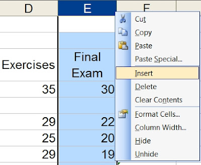
Enter the column heading Assignments. Change the new column width if necessary. Enter the new column values of 40; 32, 30, 35, 28, 22,17, 25, 22, 29, 31, 33,16. Update the cell formats to match the current formats.
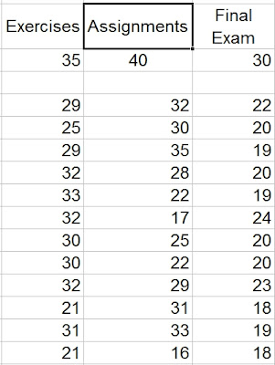
4. Add a new column heading in cell H6 called Student %.
5. In cell H9, calculate the Student % for his/her total mark. The formula to calculate the percent is the Student Total Mark divided by the Total. Set the Total cell as an absolute cell in the formula.
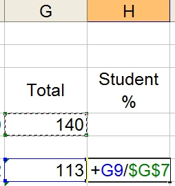
Format the result to % with 0 decimal places. Copy the formula down.
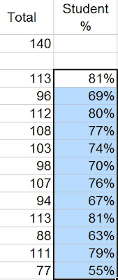
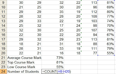
6. At the bottom of the spreadsheet in column A, add 4 new row labels Average Course Mark, Top Course Mark, Low Course Mark and Number of Students.
Use functions that will calculate the above figures for column H only. Format the answers to match the rest of the columns.
7. Change the page orientation to landscape. Center the spreadsheet horizontally and vertically on the page.
8. IMPORTANT - Use the SAVE AS command to save the spreadsheet file as Excel ex9.